DFTB+ socket coupling with MaxwellLink

This notebook shows how to run real-time TDDFTB dynamics by connecting a modified DFTB+ code (https://github.com/TEL-Research/dftbplus) to MaxwellLink.

Overall, to enable the coupling between DFTB+ with MaxwellLink, add the following MaxwellLinkSocket block within ElectronDynamics:

ElectronDynamics = {
  ...
  MaxwellLinkSocket = {
    File = "__MXL_SOCKET__"
    ResetDipole = Yes
  }
}

Here, we use the UNIX socket communication between the DFTB+ code and MaxwellLink.

To make our life simple, here we focus on:

• A single H2 molecule forming electronic strong coupling in a single-mode cavity without the dipole self-energy term.

In this case, nuclear motion is enabled and the initial temperature is set as 0 K.

from pathlib import Path
import os
import shutil
import subprocess
import time

import matplotlib.pyplot as plt
import numpy as np

import maxwelllink as mxl
from maxwelllink.tools import ir_spectrum, rt_tddft_spectrum

ROOT = Path.cwd()
INPUT_DIR = ROOT / "dftbplus_input"
RUN_ROOT = ROOT / "dftbplus_runs"
RUN_ROOT.mkdir(exist_ok=True)

AU_TO_CM = 219474.6313705
AU_TO_EV = 27.211386245988
AU_TO_FS = 0.024188843265857

DFTBPLUS_BIN = os.environ.get("DFTBPLUS_BIN") or shutil.which("dftb+")
if DFTBPLUS_BIN is None:
    raise RuntimeError("Could not find DFTB+. Set DFTBPLUS_BIN to a socket-enabled dftb+ executable.")

print("Using DFTB+:", DFTBPLUS_BIN)


def normalize_spectrum(sp):
    sp = np.asarray(sp, dtype=float)
    scale = np.nanmax(np.abs(sp)) if sp.size else 0.0
    return sp / scale if scale > 0.0 else sp


def fft_spectrum_cm(signal, dt_au):
    signal = np.asarray(signal, dtype=float)
    centered = signal - np.mean(signal)
    window = np.hanning(centered.size)
    spectrum = np.abs(np.fft.rfft(centered * window)) ** 2
    omega_au = 2.0 * np.pi * np.fft.rfftfreq(centered.size, d=dt_au)
    return omega_au[1:] * AU_TO_CM, spectrum[1:]

Using DFTB+: /Users/taoli/.local/bin/dftb+

1. Prepare and launch DFTB+

The template h2_electronic_socket.hsd in dftbplus_input/ is based on the standard DFTB+ H2 real-time singlet test. The helper functions below supplies the DFTB+ H2 input file with runtime parameters.

def prepare_h2_electronic_run(socket_name: str, dt_au_value: float, steps: int):
    run_dir = RUN_ROOT / "h2_electronic_no_dse"
    run_dir.mkdir(parents=True, exist_ok=True)

    text = (INPUT_DIR / "h2_electronic_socket.hsd").read_text()
    text = text.replace("__MXL_SOCKET__", socket_name)
    text = text.replace("__DT_AU__", f"{dt_au_value:.16e}")
    text = text.replace("__STEPS__", str(int(steps)))
    (run_dir / "dftb_in.hsd").write_text(text)

    shutil.copy2(INPUT_DIR / "H-H.skf", run_dir / "H-H.skf")
    return run_dir


def launch_h2_electronic_dftb(run_dir: Path, sleep_time: float = 0.5):
    stdout = open(run_dir / "dftbplus.out", "w")
    print("Launching DFTB+ in", run_dir)
    proc = subprocess.Popen(
        [DFTBPLUS_BIN],
        cwd=run_dir,
        stdout=stdout,
        stderr=subprocess.STDOUT,
    )
    time.sleep(sleep_time)
    if proc.poll() is not None:
        stdout.close()
        tail = (run_dir / "dftbplus.out").read_text(errors="replace")[-4000:]
        raise RuntimeError(f"DFTB+ exited before socket coupling started. Tail of dftbplus.out:\n{tail}")
    return proc, stdout

2. Run the coupled electronic simulation

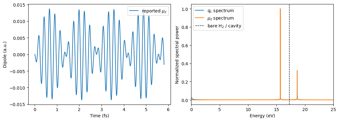
The DFTB+ electronic timestep and the MaxwellLink timestep are both 0.2 au. The approximate H2 electronic resonance used here is 17.2 eV. Here, we assume an initially purturbed cavity coordinate coupled to a ground-state H2 molecule.

socket_h2 = "dftbplus_h2_electronic"
h2_dt_au = 0.2
h2_steps = 1200
h2_resonance_ev = 17.2
h2_frequency_au = h2_resonance_ev / AU_TO_EV

hub_h2 = mxl.SocketHub(unixsocket=socket_h2, timeout=20.0, latency=1e-5)
mol_h2 = mxl.Molecule(hub=hub_h2, rescaling_factor=1.0)

sim_h2 = mxl.SingleModeSimulation(
    hub=hub_h2,
    molecules=[mol_h2],
    frequency_au=h2_frequency_au,
    coupling_strength=5e-2,
    damping_au=0.0,
    coupling_axis="z",
    drive=0.0,
    dt_au=h2_dt_au,
    qc_initial=[0.0, 0.0, 1e-2],
    record_history=True,
    include_dse=False,
)

run_h2 = prepare_h2_electronic_run(socket_h2, h2_dt_au, h2_steps)
proc_h2, stdout_h2 = launch_h2_electronic_dftb(run_h2)
sim_h2.run(steps=h2_steps)

print("DFTB+ run directory:", run_h2)

[Init Molecule] Under socket mode, registered molecule with ID 0
Launching DFTB+ in /Users/taoli/Documents/Github/MaxwellLink/tutorials/dftbplus_runs/h2_electronic_no_dse
[SocketHub] CONNECTED: mol 0 <-
[SingleModeCavity] Completed 1000/1200 [83.3%] steps, time/step: 8.30e-04 seconds, remaining time: 0.17 seconds.
[SocketHub] DISCONNECTED: mol 0 from
[SocketHub] Unlinked unix socket path /tmp/socketmxl_dftbplus_h2_electronic
DFTB+ run directory: /Users/taoli/Documents/Github/MaxwellLink/tutorials/dftbplus_runs/h2_electronic_no_dse

3. Plot the electronic polariton spectrum and energy trace

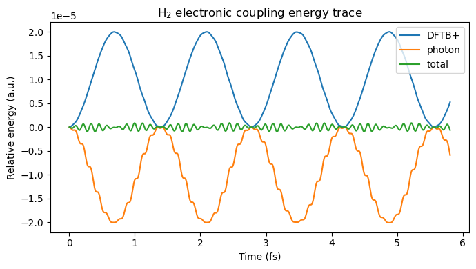
Below we show the simulation results for the photonic coordinate and the DFTB+ dipole dynamics as well as their spectra. Energy conservation is also evaluated for checking the correctness of implementation.

history_h2 = mol_h2.additional_data_history
t_h2_au = np.array([ad["time_au"] for ad in history_h2])
t_h2_fs = t_h2_au * AU_TO_FS
muz_h2 = np.array([ad["muz_au"] for ad in history_h2])
muz_h2_mid = np.array([ad.get("muz_m_au", ad["muz_au"]) for ad in history_h2])
qc_h2_z = np.array([q[2] for q in sim_h2.qc_history[: len(history_h2)]])

nskip_h2 = 5
freq_qc_ev, sp_qc_h2, _, _ = rt_tddft_spectrum(
    qc_h2_z[::nskip_h2],
    dt_au=sim_h2.dt * nskip_h2,
    sp_form="absolute",
    e_start_ev=0.1,
    e_cutoff_ev=25.0,
    sigma=1.0e5,
    w_step=2.0e-4,
)
freq_mu_ev, sp_mu_h2, _, _ = rt_tddft_spectrum(
    muz_h2[::nskip_h2],
    dt_au=sim_h2.dt * nskip_h2,
    sp_form="absolute",
    e_start_ev=0.1,
    e_cutoff_ev=25.0,
    sigma=1.0e5,
    w_step=2.0e-4,
)

fig, ax = plt.subplots(1, 2, figsize=(11, 4))
ax[0].plot(t_h2_fs, muz_h2, label=r"reported $\mu_z$")
ax[0].set_xlabel("Time (fs)")
ax[0].set_ylabel("Dipole (a.u.)")
ax[0].legend()

ax[1].plot(freq_qc_ev, normalize_spectrum(sp_qc_h2), label="$q_c$ spectrum")
ax[1].plot(freq_mu_ev, normalize_spectrum(sp_mu_h2), label=r"$\mu_z$ spectrum")
ax[1].axvline(h2_resonance_ev, color="k", ls="--", lw=1.0, label="bare H$_2$ / cavity")
ax[1].set_xlim(0, 25)
ax[1].set_xlabel("Energy (eV)")
ax[1].set_ylabel("Normalized spectral power")
ax[1].legend()
plt.tight_layout()
plt.show()

energy_molecule_h2 = np.array([ad["energy_au"] for ad in history_h2])
energy_total_h2 = np.array(sim_h2.energy_history[: len(history_h2)])
energy_photon_h2 = energy_total_h2 - energy_molecule_h2

plt.figure(figsize=(7, 4))
plt.plot(t_h2_fs, energy_molecule_h2 - energy_molecule_h2[0], label="DFTB+")
plt.plot(t_h2_fs, energy_photon_h2 - energy_photon_h2[0], label="photon")
plt.plot(t_h2_fs, energy_total_h2 - energy_total_h2[0], label="total")
plt.xlabel("Time (fs)")
plt.ylabel("Relative energy (a.u.)")
plt.title("H$_2$ electronic coupling energy trace")
plt.legend()
plt.tight_layout()
plt.show()