Driven dynamics with TLS

Here, we demonstrate the socket-free TLS workflow using the maxwelllink.LaserDrivenSimulation electromagnetic solver. By resonantly coupling one cosine driving field to a two-level system (TLS), we aim to monitor the driven population dynamics of the TLS.

1. Defining Molecule

We first create a Molecule instance using the non-socket mode, i.e., we directly initialize the TLS within the Molecule class:

import numpy as np
import maxwelllink as mxl

frequency_au = 1.0
mu12 = 1

molecule = mxl.Molecule(
    driver="tls",
    driver_kwargs={
        "omega": frequency_au,
        "mu12": mu12,
        "orientation": 2,
        "pe_initial": 0e-3,
    }
)

[Init Molecule] Operating in non-socket mode, using driver: tls

2. Defining the driven field

Then, we create a LaserDrivenSimulation instance which defines the parameters for a custom driven field. The pre-defined molecule is also attached to this class for coupled light-matter simulations.

from maxwelllink.tools import cosine_drive

dt_au = 1e-1
total_steps = 2e4

# you are encouraged to try different field parameters
omega_au_field = frequency_au * 1.0
amplitude_au = 1e-2

sim = mxl.LaserDrivenSimulation(
    molecules=[molecule],
    coupling_axis="z",
    drive=cosine_drive(omega_au=omega_au_field, amplitude_au=amplitude_au),
    dt_au=dt_au,
    record_history=True,
)

sim.run(steps=total_steps)

init TLSModel with dt = 0.100000 a.u., molecule ID = 0
[LaserDriven] Completed 1000/20000.0 [5.0%] steps, time/step: 9.14e-05 seconds, remaining time: 1.74 seconds.
[LaserDriven] Completed 2000/20000.0 [10.0%] steps, time/step: 2.15e-04 seconds, remaining time: 2.76 seconds.
[LaserDriven] Completed 3000/20000.0 [15.0%] steps, time/step: 1.35e-04 seconds, remaining time: 2.50 seconds.
[LaserDriven] Completed 4000/20000.0 [20.0%] steps, time/step: 8.59e-05 seconds, remaining time: 2.11 seconds.
[LaserDriven] Completed 5000/20000.0 [25.0%] steps, time/step: 8.76e-05 seconds, remaining time: 1.84 seconds.
[LaserDriven] Completed 6000/20000.0 [30.0%] steps, time/step: 8.45e-05 seconds, remaining time: 1.63 seconds.
[LaserDriven] Completed 7000/20000.0 [35.0%] steps, time/step: 1.09e-04 seconds, remaining time: 1.50 seconds.
[LaserDriven] Completed 8000/20000.0 [40.0%] steps, time/step: 1.02e-04 seconds, remaining time: 1.37 seconds.
[LaserDriven] Completed 9000/20000.0 [45.0%] steps, time/step: 9.78e-05 seconds, remaining time: 1.23 seconds.
[LaserDriven] Completed 10000/20000.0 [50.0%] steps, time/step: 9.01e-05 seconds, remaining time: 1.10 seconds.
[LaserDriven] Completed 11000/20000.0 [55.0%] steps, time/step: 8.25e-05 seconds, remaining time: 0.97 seconds.
[LaserDriven] Completed 12000/20000.0 [60.0%] steps, time/step: 8.30e-05 seconds, remaining time: 0.84 seconds.
[LaserDriven] Completed 13000/20000.0 [65.0%] steps, time/step: 9.35e-05 seconds, remaining time: 0.73 seconds.
[LaserDriven] Completed 14000/20000.0 [70.0%] steps, time/step: 8.52e-05 seconds, remaining time: 0.62 seconds.
[LaserDriven] Completed 15000/20000.0 [75.0%] steps, time/step: 8.39e-05 seconds, remaining time: 0.51 seconds.
[LaserDriven] Completed 16000/20000.0 [80.0%] steps, time/step: 9.48e-05 seconds, remaining time: 0.41 seconds.
[LaserDriven] Completed 17000/20000.0 [85.0%] steps, time/step: 8.19e-05 seconds, remaining time: 0.30 seconds.
[LaserDriven] Completed 18000/20000.0 [90.0%] steps, time/step: 8.43e-05 seconds, remaining time: 0.20 seconds.
[LaserDriven] Completed 19000/20000.0 [95.0%] steps, time/step: 8.75e-05 seconds, remaining time: 0.10 seconds.
[LaserDriven] Completed 20000/20000.0 [100.0%] steps, time/step: 8.48e-05 seconds, remaining time: 0.00 seconds.

3. Retrieve simulation observables

After the simulation, we can retrieve the TLS trajectory from molecule.extra.

# users can also use molecule.additional_data_history to access the time-resolved data recorded during the simulation,
# population = np.array([entry["Pe"] for entry in molecule.additional_data_history])
# tls_time_au = np.array([entry["time_au"] for entry in molecule.additional_data_history])
# but here we demonstrate the use of molecule.extra which is more convenient for post-processing and plotting.
population = molecule.extra["Pe"]
tls_time_au = molecule.extra["time_au"]

print(
    f"Collected {population.size} TLS samples."
)

Collected 20000 TLS samples.

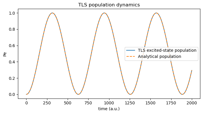
4. Inspect time-domain Rabi oscillations

According to the analytical rotating wave approximation, under near resonance excitation, the excited-state population \(P_{\rm e}(t)\) obeys:

\[P_{\rm e}(t) = \frac{\Omega_0^2}{\Omega_{\rm R}^2} \sin^2(\frac{\Omega_{\rm R} t}{2}).\]

where \(\Omega_0 \equiv \mu_{12} E_0\) and \(\Omega_{\rm R} = \sqrt{\Delta^2 + \Omega_0^2}\), with \(\Delta = \omega_0 - \omega_{\rm {ph}}\) denoting the light-matter detuning.

import matplotlib.pyplot as plt

# analytical solution under RWA
Omega_0 = mu12 * amplitude_au
Omega_R = np.sqrt(Omega_0**2 + (omega_au_field - frequency_au) ** 2)
population_analytical = Omega_0**2 / Omega_R**2 * np.sin(Omega_R * tls_time_au / 2) ** 2

plt.figure(figsize=(7, 4))
plt.plot(tls_time_au, population, label="TLS excited-state population")
plt.plot(tls_time_au, population_analytical, label="Analytical population", linestyle="--")
plt.xlabel("time (a.u.)")
plt.ylabel("Pe")
plt.title("TLS population dynamics")
plt.legend()
plt.tight_layout()
plt.show()