Introduction to real-time time-dependent Hartree-Fock theory
This notebook is written for graduate students who already understand the two-level system (TLS) and want to make the conceptual jump to real-time mean-field electronic dynamics in molecules.
We take \(\rm{H}_2\), the smallest closed-shell molecule, as an example.
0. Roadmap: from a two-level system to many-electron mean field
Recall the canonical TLS:
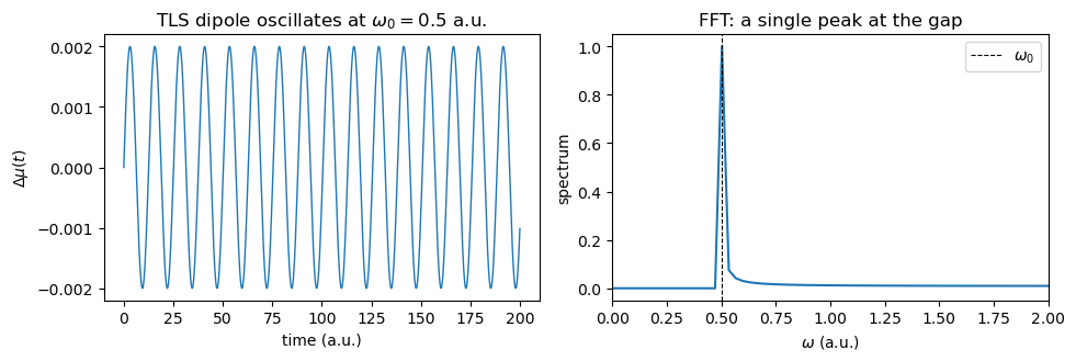
A weak delta kick along the dipole, \(U_{\text{kick}} = e^{\,i\kappa\hat\mu}\), prepares a small coherence between the two eigenstates. The induced dipole then oscillates,
and its FFT yields a single peak at \(\omega = \omega_0\).
Real-time time-dependent Hartree–Fock (RT-TDHF) applies the same idea to a many-electron system.
Below is the comparison between TLS dynamics and RT-TDHF:
concept |
TLS |
RT-TDHF |
|---|---|---|
state |
\(\rho\) (\(2\times 2\)) |
density matrix \(P\) in the AO basis (\(N\times N\)) |
Hamiltonian |
\(H_0\) (constant) |
Fock \(F[P] = H_{\text{core}}+J[P]-\tfrac12 K[P]\) (depends on \(P\)!) |
equation of motion |
\(i\dot\rho=[H_0,\rho]\) |
\(i\dot P=[F[P],P]\) (Liouville–von Neumann, nonlinear) |
dipole operator |
\(\mu_0\sigma_x\) |
AO matrix \(\boldsymbol\mu = -\mathbf r\) (electronic) + nuclei |
eigenbasis |
\(\sigma_z\) basis |
orthogonal AO basis using \(X = S^{-1/2}\) transform |
linear-response peaks |
one, at \(\omega_0\) |
many, such as bonding→antibonding (\(\sigma\to\sigma^*\)). |
The only non-trivial twist is the second row: in mean-field electronic theory, the effective Hamiltonian \(F[P]\) depends on the state \(P\) itself. In Hartree-Fock theory, as electrons feel the average potential of all other electrons, the Hamiltonian becomes nonlinear, which makes it difficult to maintain the stability of numerical propagation as a function of time.
1. Recall the TLS dynamics
Before moving to \(\rm{H}_2\), let us run the time-resolved dynamics for a single TLS.
[1]:
import numpy as np
from scipy.linalg import expm
import matplotlib.pyplot as plt

omega0    = 0.5      # TLS gap (a.u.)
mu0       = 1.0      # transition dipole (a.u.)
kappa_tls = 1.0e-3   # weak kick
dt_tls    = 0.05
nstep_tls = 4000

# 1. Hamiltonian and dipole operator
H0 = 0.5 * omega0 * np.array([[ 1, 0], [ 0,-1]], dtype=complex)   # sigma_z
mu_op = mu0       * np.array([[ 0, 1], [ 1, 0]], dtype=complex)   # sigma_x

# 2. Ground state density: |1><1| (lower eigenstate of sigma_z)
rho = np.array([[0, 0], [0, 1]], dtype=complex)

# 3. Delta kick: rho -> exp(+i kappa mu) rho exp(-i kappa mu)
U_kick = expm(1j * kappa_tls * mu_op)
rho = U_kick @ rho @ U_kick.conj().T

# 4. Field-free unitary propagation: rho -> exp(-i H0 dt) rho exp(+i H0 dt)
U_dt = expm(-1j * dt_tls * H0)
times_tls, dip_tls = [0.0], [np.trace(mu_op @ rho).real]
for n in range(1, nstep_tls + 1):
    rho = U_dt @ rho @ U_dt.conj().T
    times_tls.append(n * dt_tls)
    dip_tls.append(np.trace(mu_op @ rho).real)
times_tls = np.array(times_tls)
dip_tls   = np.array(dip_tls) - dip_tls[0]

# 5. FFT of the induced dipole
sig_tls = dip_tls * np.exp(-1e-3 * times_tls)
fft_tls = np.fft.rfft(sig_tls)
omega_tls = 2.0 * np.pi * np.fft.rfftfreq(sig_tls.size, d=dt_tls)
spec_tls  = -omega_tls * fft_tls.imag
spec_tls  = np.clip(spec_tls / (np.abs(spec_tls).max() + 1e-30), 0.0, None)

fig, ax = plt.subplots(1, 2, figsize=(10, 3.4))
ax[0].plot(times_tls, dip_tls, lw=1)
ax[0].set(xlabel="time (a.u.)", ylabel=r"$\Delta\mu(t)$",
          title=fr"TLS dipole oscillates at $\omega_0={omega0}$ a.u.")
ax[1].plot(omega_tls, spec_tls, lw=1.5)
ax[1].axvline(omega0, color="k", ls="--", lw=0.8, label=r"$\omega_0$")
ax[1].set(xlim=(0, 2), xlabel=r"$\omega$ (a.u.)", ylabel="spectrum",
          title="FFT: a single peak at the gap"); ax[1].legend()
plt.tight_layout(); plt.show()
2. The same procedure for \(\rm{H}_2\)
Below are the equations we will implement. Compare each line with the TLS dynamics just above.
Closed-shell Fock matrix (the analog of \(H_0\), but state-dependent):
Symmetric orthogonalization (going to a clean “basis”, because atomic orbitals, or AOs, are not orthogonal):
Delta kick (identical operator structure as in the TLS):
Unitary propagation in the orthogonal basis (TLS analog: \(e^{-iH_0\Delta t}\)):
Spectrum (identical formula to the TLS):
The single new ingredient compared to the TLS is that :math:`F` is rebuilt from :math:`P` at every step.
[2]:
import numpy as np
import psi4
import matplotlib.pyplot as plt
from scipy.linalg import expm, fractional_matrix_power

# Unit conversions
au_to_fs = 0.024188843265857
hartree_to_ev = 27.211386245988

# Simulation parameters
R_angstrom = 0.74        # H-H bond length
dt = 0.04                # time step in atomic units
nsteps = 1200            # total number of propagation steps
kappa = 1.0e-3           # delta-kick strength (a.u.)
eta = 1.0e-3             # optional exponential damping for FFT (a.u.^-1)

# Make plots a bit larger
plt.rcParams["figure.figsize"] = (7, 4)
plt.rcParams["font.size"] = 12
3. Step 1 - Ground state: solve RHF to get \(P_0\)
In the TLS we picked the ground state \(|1\rangle\langle 1|\) by hand. For a real molecule we have to solve the static problem first: a self-consistent diagonalization of \(F[P]\), i.e. ordinary RHF.
We place \(\rm{H}_2\) along the \(z\) axis with the bond midpoint at the origin so that the permanent dipole is zero by symmetry.
[3]:
psi4.core.clean()
psi4.set_memory("1 GB")
psi4.core.set_num_threads(1)
psi4.core.set_output_file("psi4_h2_rt_tdhf.out", False)

mol = psi4.geometry(f'''
units angstrom
nocom
noreorient
symmetry c1
0 1
H 0.0 0.0 {-R_angstrom/2.0}
H 0.0 0.0 {+R_angstrom/2.0}
''')

psi4.set_options({
    "basis": "cc-pvdz",
    "reference": "rhf",
    "scf_type": "pk",
    "e_convergence": 1e-12,
    "d_convergence": 1e-12,
})

E_scf, wfn = psi4.energy("scf", return_wfn=True)
print(f"Ground-state RHF energy = {E_scf:.12f} Eh")
  Memory set to 953.674 MiB by Python driver.
  Threads set to 1 by Python driver.
Ground-state RHF energy = -1.128700093561 Eh
4. Step 2 - Build \(F\), \(\boldsymbol\mu\), and the orthogonalizer
The “Hamiltonian” of an electronic problem in a finite AO basis is the Fock matrix \(F[P]\). Building it requires:
the overlap \(S\) (because AOs are not orthogonal),
the core Hamiltonian \(H_{\text{core}}\) (kinetic + electron–nucleus),
the two-electron integrals \((\mu\nu|\rho\sigma)\), from which \(J[P]\) and \(K[P]\) are contracted at every step,
the dipole integrals, which become the AO matrix of \(\hat\mu\).
We then build \(X=S^{-1/2}\) once. Multiplying by \(X\) on both sides plays the same role as moving a TLS Hamiltonian into the basis where \(\sigma_z\) is diagonal: in that basis the propagator has the simple form \(P\to e^{-iF\Delta t}\,P\,e^{+iF\Delta t}\).
[4]:
mints = psi4.core.MintsHelper(wfn.basisset())

S = np.asarray(wfn.S())
Hcore = np.asarray(wfn.H())
ERI = np.asarray(mints.ao_eri())

# Psi4 returns position integrals <chi_mu | x,y,z | chi_nu>.
# The electronic dipole operator is -r, so we add the minus sign here.
x_ao, y_ao, z_ao = [np.asarray(m) for m in mints.ao_dipole()]
mu_x_ao = -x_ao
mu_y_ao = -y_ao
mu_z_ao = -z_ao

# Closed-shell total density P = 2 * D_alpha (density matrix of the alpha electron)
P0 = 2.0 * np.asarray(wfn.Da())

# Symmetric orthogonalization matrices
X = fractional_matrix_power(S, -0.5)
U = fractional_matrix_power(S,  0.5)

# Nuclear dipole (in a.u.); for midpoint-centered H2 this is zero
R_bohr = np.array([[mol.x(A), mol.y(A), mol.z(A)] for A in range(mol.natom())])
Z = np.array([mol.Z(A) for A in range(mol.natom())])
mu_nuc = (Z[:, None] * R_bohr).sum(axis=0)

print("Number of AO functions =", S.shape[0])
print("Ground-state total dipole (a.u.) =", np.trace(P0 @ mu_z_ao).real + mu_nuc[2])
Number of AO functions = 10
Ground-state total dipole (a.u.) = 3.497202527569243e-15
Inspect the orbital structure: the closest analog of \(\omega_0\)
The bare HOMO–LUMO gap is the simplest analog of the TLS gap \(\omega_0\). But the actual RT-TDHF (and LR-TDHF) excitation energy is shifted from this gap by the electron–electron interaction in \(J[P]-\tfrac12K[P]\).
[5]:
eps = np.asarray(wfn.epsilon_a())
nocc = wfn.nalpha()  # number of doubly-occupied MOs (= 1 for H2)

print(f"All MO energies (Eh):")
for i, e in enumerate(eps):
    label = "HOMO" if i == nocc - 1 else "LUMO" if i == nocc else "    "
    print(f"  MO {i:2d}  {label}  e = {e: .5f} Eh")

gap = eps[nocc] - eps[nocc - 1]
print(f"\nHOMO–LUMO gap = {gap:.4f} Eh = {gap*hartree_to_ev:.3f} eV")
print("\nWe will see below that the lowest RT-TDHF / LR-TDHF peak is *not*")
print("at this bare gap. Instead, it is shifted by electron-electron interactions,")
print("which is precisely the nonlinear part of F[P].")
All MO energies (Eh):
  MO  0  HOMO  e = -0.59241 Eh
  MO  1  LUMO  e =  0.19744 Eh
  MO  2        e =  0.47932 Eh
  MO  3        e =  0.93732 Eh
  MO  4        e =  1.29290 Eh
  MO  5        e =  1.29290 Eh
  MO  6        e =  1.95702 Eh
  MO  7        e =  2.04352 Eh
  MO  8        e =  2.04352 Eh
  MO  9        e =  3.61047 Eh

HOMO–LUMO gap = 0.7899 Eh = 21.493 eV

We will see below that the lowest RT-TDHF / LR-TDHF peak is *not*
at this bare gap. Instead, it is shifted by electron-electron interactions,
which is precisely the nonlinear part of F[P].
[6]:
def build_fock(P):
    """Closed-shell RHF Fock matrix built from the total AO density P."""
    J = np.einsum("pqrs,rs->pq", ERI, P, optimize=True)
    K = np.einsum("prqs,rs->pq", ERI, P, optimize=True)
    F = Hcore + J - 0.5 * K
    return 0.5 * (F + F.conj().T)


def ao_to_orth_density(P):
    return U @ P @ U.conj().T


def orth_to_ao_density(P_orth):
    return X @ P_orth @ X.conj().T


def ao_to_orth_operator(A):
    return X.conj().T @ A @ X


def dipole_z(P):
    """Total molecular dipole along z (electrons + nuclei)."""
    return np.trace(P @ mu_z_ao).real + mu_nuc[2]


def rhf_energy(P, F):
    """Closed-shell RHF total energy from the total density P."""
    return 0.5 * np.trace(P @ (Hcore + F)).real + mol.nuclear_repulsion_energy()
5. Step 3 - Kick the molecule (same operator as in the TLS)
In the TLS we applied \(e^{i\kappa\sigma_x}\) to the ground state. Here we apply \(e^{i\kappa\hat\mu_z}\) to the orthogonalized density, which generates a small coherence between every occupied MO and every virtual MO with non-zero \(z\)-dipole matrix element to it (in \(\rm{H}_2\), the dominant channel is \(\sigma_g \to \sigma_u^*\)).
Because \(\kappa\) is small, we stay in the linear-response regime: the Fourier transform of \(\Delta\mu_z(t)\) samples the linear-response polarizability \(\alpha_{zz}(\omega)\).
[7]:
P0_orth = ao_to_orth_density(P0)
mu_z_orth = ao_to_orth_operator(mu_z_ao)

U_kick = expm(1j * kappa * mu_z_orth)
P_kicked_orth = U_kick @ P0_orth @ U_kick.conj().T
P_kicked = orth_to_ao_density(P_kicked_orth)
P_kicked = 0.5 * (P_kicked + P_kicked.conj().T)

print(f"Induced dipole immediately after the kick = {dipole_z(P_kicked): .6e} a.u.")
Induced dipole immediately after the kick = 3.941292e-15 a.u.
6. Step 4 - Real-time propagation
We use the simplest possible scheme: at each step, build \(F\) from the current \(P\), then take a unitary step
This is first-order accurate because \(F\) is evaluated at the start of the step. In other words, the energy drift following this unitary propagation scheme scales in the order of \(\Delta t\).
For improving the energy conservation, a midpoint or modified-midpoint scheme (the “MMUT” propagator used in production codes) can be applied, but this is outside the scope of this tutorial.
[8]:
import numpy as np
from scipy.linalg import expm

def propagate_naive_unitary(P_start_orth, dt, nsteps):
    """Naive first-order RT-TDHF propagation in the orthonormal basis.

    Propagation rule:
        F_n = F[P_n]
        U_n = exp(-i dt F_n)
        P_{n+1} = U_n P_n U_n^dagger

    This is simpler than MMUT because it does not use a midpoint density or
    half-step bootstrap. It is unitary, but only first-order accurate in time
    for nonlinear TDHF.
    """

    # Initial density
    P_orth = P_start_orth.copy()
    P_orth = 0.5 * (P_orth + P_orth.conj().T)

    # Initial AO density and observables
    P_ao = orth_to_ao_density(P_orth)
    P_ao = 0.5 * (P_ao + P_ao.conj().T)

    F_ao = build_fock(P_ao)
    F_ao = 0.5 * (F_ao + F_ao.conj().T)

    times = [0.0]
    dipoles = [dipole_z(P_ao)]
    energies = [rhf_energy(P_ao, F_ao)]

    for step in range(1, nsteps + 1):
        # Fock from the density at the beginning of the step
        P_ao = orth_to_ao_density(P_orth)
        P_ao = 0.5 * (P_ao + P_ao.conj().T)

        F_ao = build_fock(P_ao)
        F_ao = 0.5 * (F_ao + F_ao.conj().T)

        F_orth = ao_to_orth_operator(F_ao)
        F_orth = 0.5 * (F_orth + F_orth.conj().T)

        # Naive full-step unitary propagation
        U_step = expm(-1j * dt * F_orth)
        P_orth = U_step @ P_orth @ U_step.conj().T
        P_orth = 0.5 * (P_orth + P_orth.conj().T)

        # Back to AO basis for analysis
        P_ao = orth_to_ao_density(P_orth)
        P_ao = 0.5 * (P_ao + P_ao.conj().T)

        F_ao = build_fock(P_ao)
        F_ao = 0.5 * (F_ao + F_ao.conj().T)

        times.append(step * dt)
        dipoles.append(dipole_z(P_ao))
        energies.append(rhf_energy(P_ao, F_ao))

    return np.array(times), np.array(dipoles), np.array(energies)
[9]:
times_au, dipoles_z, energies = propagate_naive_unitary(P_kicked_orth, dt, nsteps)
times_fs = times_au * au_to_fs

print(f"Total propagation time = {times_fs[-1]:.3f} fs")
print(f"Max energy drift       = {np.max(np.abs(energies - energies[0])):.3e} Eh")
Total propagation time = 1.161 fs
Max energy drift       = 3.190e-07 Eh
[10]:
delta_mu = dipoles_z - dipoles_z[0]

plt.plot(times_fs, delta_mu, lw=1.0)
plt.xlabel("Time (fs)")
plt.ylabel(r"$\Delta \mu_z(t)$ (a.u.)")
plt.title("Induced dipole after a delta kick")
plt.tight_layout()
plt.show()
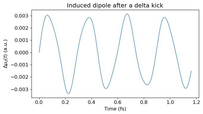
Here, just like the TLS dynamics, \(\Delta\mu_z(t)\) is a small oscillation around zero. However, unlike the TLS, it is not a single sinusoid: it is a sum of contributions from every dipole-allowed excitation that the kick excited.
7. Step 5 - Spectrum from the dipole trajectory
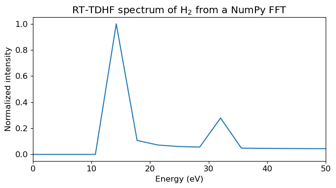
The FFT step is identical to the TLS procedure. The damping factor \(e^{-\eta t}\) below broadens the discrete peaks into Lorentzians.
The absorption-like spectrum is
The factor of \(\omega\) is the standard convention that turns the polarizability into an oscillator-strength-like quantity.
[11]:
signal = delta_mu * np.exp(-eta * times_au)

fft_vals = np.fft.rfft(signal)
omega_au = 2.0 * np.pi * np.fft.rfftfreq(signal.size, d=dt)
energy_ev = omega_au * hartree_to_ev

# A simple absorption-like spectrum from the NumPy FFT.
alpha_w = (dt / kappa) * fft_vals
spectrum = omega_au * (-alpha_w.imag)

# Clean up the zero-frequency point and any tiny negative noise
spectrum[0] = 0.0
spectrum = np.clip(spectrum, 0.0, None)

# Normalize for plotting
if spectrum.max() > 0:
    spectrum = spectrum / spectrum.max()
[12]:
plt.plot(energy_ev, spectrum, lw=1.5)
plt.xlim(0, 50)
plt.xlabel("Energy (eV)")
plt.ylabel("Normalized intensity")
plt.title("RT-TDHF spectrum of H$_2$ from a NumPy FFT")
plt.tight_layout()
plt.show()
8. Cross-check: linear response TDHF (LR-TDHF)
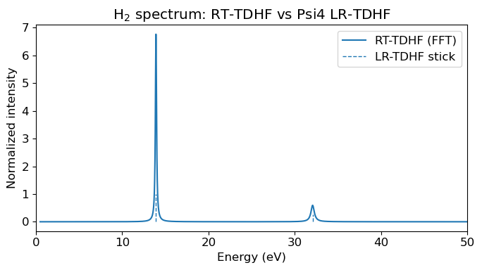
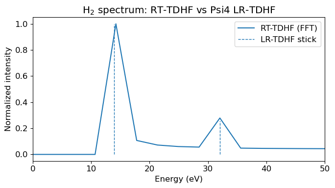
LR-TDHF solves an eigenvalue problem for the linear response of the same Fock operator. In the weak-kick limit, RT-TDHF and LR-TDHF must predict the same excitation energies and oscillator strengths. The peak positions in our spectrum should line up with the LR-TDHF stick spectrum.
[13]:
from psi4.driver.procrouting.response.scf_response import tdscf_excitations

psi4.set_options({
    "basis": "cc-pvdz",
    "reference": "rhf",
    "scf_type": "pk",
    "save_jk": True,
})

E_lr, wfn_lr = psi4.energy("scf", return_wfn=True, molecule=mol)
lr_res = tdscf_excitations(wfn_lr, states=3, tda=False)

exc_ev = np.array([r["EXCITATION ENERGY"] for r in lr_res]) * hartree_to_ev
osc = np.array([r["OSCILLATOR STRENGTH (LEN)"] for r in lr_res])

print("LR-TDHF excitation energy (eV):", exc_ev)
print("LR-TDHF oscillator strength:", osc)

plt.plot(energy_ev, spectrum, label="RT-TDHF (FFT)")
plt.vlines(exc_ev, 0, osc/np.max(osc), linestyles="dashed", linewidth=1.0, label="LR-TDHF stick")
plt.xlim(0, 50)
plt.xlabel("Energy (eV)")
plt.ylabel("Normalized intensity")
plt.title("H$_2$ spectrum: RT-TDHF vs Psi4 LR-TDHF")
plt.legend()
plt.tight_layout()
plt.show()
LR-TDHF excitation energy (eV): [13.91137134 21.31926952 32.05653779]
LR-TDHF oscillator strength: [0.53262017 0.         0.13572863]
9. Padé FFT in MaxwellLink: a shorter trajectory suffices
A plain FFT needs a long trajectory to resolve sharp peaks: the spectral resolution is \(\Delta\omega \sim 2\pi / T_{\text{total}}\). The Padé approximant rewrites the FFT as a rational function and converges much faster, so you can extract clean peaks from a shorter trajectory at the cost of slightly biased line shapes. This Padé function is shipped within MaxwellLink.
[14]:
from maxwelllink.tools import rt_tddft_spectrum

# call Pade approximation FFT spectrum function
freq_ev, sp_tot, t_fs, mu = rt_tddft_spectrum(delta_mu, dt, e_cutoff_ev=50)

plt.plot(freq_ev, sp_tot, label="RT-TDHF (FFT)")
plt.vlines(exc_ev, 0, osc/np.max(osc), linestyles="dashed", linewidth=1.0, label="LR-TDHF stick")
plt.xlim(0, 50)
plt.xlabel("Energy (eV)")
plt.ylabel("Normalized intensity")
plt.title("H$_2$ spectrum: RT-TDHF vs Psi4 LR-TDHF")
plt.legend()
plt.tight_layout()
plt.show()